Guidelines for using objective measures
Prerequisites for Calculations MATLAB codes have been provided to calculate values for the following metrics: Third octave band levels, loudness and sharpness. The following guidelines are also provided for the correct way to implement these codes.
For ease of calculation all editing is done prior to the MATLAB calculation using Adobe audition and instructions are provided to use Adobe audition to do this. However, any other good audio editing software could be used to adequately prepare the sound prior to the MATLAB calculation. The Sample Rate For recorded sounds the sampling rate used should be 48 kHz. If this is not the case the sounds should be resampled at the correct rate.
- Find out how to resample the sound using Adobe Audition.
The Length of the Signal
It is recommended that the original recording should be divided up into shorter duration extracts to be analysed. Each sample to be analysed must be longer than 0.5 secs in duration (to make the time delay effects of the filters negligible). 3 secs is regarded as a good length (this is 144128 samples when rounded to n x 28 samples at a sample rate of 48 kHz), though in practice this duration may depend on the original recording. More than one extract can be taken from the recording and analysed to represent different aspects of the sound. ‘Steady state’ aspects of the sound should be extracted (practical examples of this are shown in table 1).
When comparing the metrics of two or more extracts it should be ensured that each is of equal duration. Lengths of signals should be rounded to n x 28 samples to get the best performance from the metric calculators provided. For monaural sounds only one channel of the sound needs to be selected. For binaural sounds each channel need to be selected and saved to two separate .wav files. A binaural correction needs to be applied (see below) and values of the metrics for each channel should be calculated.
Aspects of the sound Number of samples taken Duration each sample Kettle Heating 1 3 secs Boiling 1 3 secs Washing Machine Washing 1 3 secs Draining 1 3 secs Spinning 7 3 secs Leaf Blower Static blowing 1 10 secs Static sucking 1 10 secs Moving blowing 1 10 secs Moving sucking 1 10 secs
Table 1: Examples of samples of domestic appliances to be analysed
- Find out how to select a signal length of n samples using Adobe Audition.
Applying the Binaural Correction
A correction needs to be applied to binaural recordings made with a head and torso simulator (HATS) before the metrics can be calculated. A ‘free field’ correction should be applied for recordings made in the anechoic chamber (this is shown in table 2 for a B&K 4100 HATS) and a ‘diffuse field’ correction should be applied for recordings made when surrounded by reflective surfaces (this is shown in table 3 for a B&K 4100 HATS). The correction should be applied to each channel, and then each channel should be extracted to a single channel .wav file.
Frequency (Hz) Correction (dB) Frequency (Hz) Correction (dB) Frequency (Hz) Correction (dB) Frequency (Hz) Correction (dB) 200 -0.03 630 -0.98 2000 -4.54 6300 -5.47 250 -0.35 800 -1.75 2500 -6.47 8000 3.34 315 -0.90 1000 -0.77 3150 -9.24 10000 -0.98 400 -1.50 1250 -2.36 4000 -13.29 12500 -4.42 500 -1.18 1600 -2.86 5000 -11.77 16000 0.70
Table 2: HATS ‘free field’ correction for a B&K 4100
Frequency (Hz) Correction (dB) Frequency (Hz) Correction (dB) Frequency (Hz) Correction (dB) Frequency (Hz) Correction (dB) 200 -0.27 630 -0.93 2000 -3.16 6300 -6.31 250 -0.33 800 -1.09 2500 -4.45 8000 -1.81 315 -0.44 1000 -1.52 3150 -6.52 10000 -0.54 400 -0.63 1250 -2.19 4000 -9.10 12500 4.32 500 -0.84 1600 -2.49 5000 -9.19 16000 9.67
Table 3: HATS ‘diffuse field’ correction for a B&K 4100
- Find out how to apply this correction using Adobe Audition