Jury testing
Asking customer’s opinions of products is a cornerstone of sound quality testing. However, this has to be done with extreme care to prevent results being biased. A major technical problem centre around context – the assessment of sound quality is very dependent on the context, for instance the expectation and emotional state of the listener. As it is impossible to remove contextual influences, the aim in drawing up a jury testing regime is to reduce and define the uncertainties introduced by the assessment regimes. It is also imperative that appropriate statistical analysis is carried out, otherwise you risk drawing incorrect conclusions from the data.
Introduction
The ultimate judgement of a product is made by people, and so in developing new products a certain amount (or maybe even a considerable amount) of testing has to be done on subjects. This is known as jury testing. The idea is to play people the sounds of the different products and get them to evaluate the quality of the sounds. However, great care must be taken when undertaking these procedures, as it is very easy to lead the subjects into making the judgements you want to hear, rather than their true opinions.
It is possible to buy sound quality testing software and hardware from an instrument manufacturer such as Bruel and Kjaer, 01dB, Head Acoustics etc.. By doing this, you buy into well made and reliable testing software. You also get all the hardware that you need, such as properly calibrated transducers. However, the cost of these instruments may be prohibitive to some, so the idea here is to give guidelines for those who want to carry out jury testing without these instruments, or to give further explanation to the process for those who own those instruments.
Why use jury testing
A jury test can allow a range of different products to be tested and to determine which one sounds the best and which the worst. For instance, what might be tested is a range of products from different manufacturers in a particular price band. By identifying the best and worst products in terms of sound, it is then possible to design products which avoid the worst sounds and make the best sounds.
Manufacturers are often motivated to look at sound quality when they find complaints from customers, maybe a product is making an annoying sound or is overly noisy. The problem can be confirmed and investigated using jury testing.
Jury testing can also be used to shape the sound to some desired characteristic. For example, to make a product sound more powerful, more robust and better made.
Sound quality assessment can also use a range of metrics to compare the sound from different products. These metrics approximately represent the human response, for example the metric loudness should correspond to people’s perception of how loud a product is. To find out which metrics are useful for which product, it is necessary to measure people’s responses to a range of sounds from a product type, and then relate (correlate) the subject’s responses to the metrics. Consequently, even if the intention in the long term is to use metrics to evaluate sound quality, in setting up the metrics, and finding out which ones are important for which products, it is necessary to undertaken jury testing.
It is also possible through jury testing to evaluate the worth of different alterations to a product to the sound produced. For example, it is possible to take a sound that a current product makes, and change this to simulate the effects of changing components in the product. By this method, it is possible to come up with the desired sound for a product before a full prototype has to be constructed.
Another approach is to develop a virtual prototype to enable predictions to be made of product sounds before physical protoypes are made. In the automobile industry, virtual protoypes are used at the early stages of the design to try and estimate what the sound quality will be like early in the design cycle, as it is easier and cheaper to alter the sound of a product if that is considered early on. Even with an existing product, simple changes can be made to the product to understand what different components are doing to change the sound quality. For example, with the kettle you could remove the lid and therefore get a sense of the effect of the air enclosure above the water [1].
1] ‘Designing for Product Sound Quality’ R.H. Lyon, (Marcel Dekker 2000)
Overview
The product is placed in a room typical of the environment where the product is normally used. The product is used and recorded via a microphone onto a digital recorder such as DAT tape. From there the sound is taken into the computer via a sound card. Once on the computer, the sound can be manipulated using commonly-available music processing software. Then the sound samples are blasted onto a CD for later reproduction The sound is then reproduced over headphones to the listener who then makes judgements on the sounds using a questionnaire.
There are many variations on the set up suggested above, but this is one of the most common.
Why carry out recordings?
It is possible to listening to one product after another “live” without recording and reproducing the sound. However, this causes many problems. For a washing machine, for example, the wash cycle is far too long for people to sit through. Even with products that have short sounds, the delay between auditioning products that happens in such “live” tests mean that the subjects’ judgements become more unreliable when comparing products. There are also products where it is difficult to ensure that each listener gets to hear the same sound because the sound is different each time the product is used. It is also important that each product is played from exactly the same position in the room, otherwise the sound is affected by the position, and so it is necessary to swap over products so they are played from the same place, and this is a slow processes for many products. For these reasons, it is best to record the sounds for later reproduction.
Recording location
The sound produced by an appliance can depend greatly on the location in which it is placed. For example below are two sounds of a kettle recorded in two very different rooms. One of them is recorded in a semi-anechoic chamber which has its surfaces covered in absorbent so you here just the sound straight from the kettle. The other is recorded in a normal kitchen. The sound quality is very different between the two sound files, and the kettle in the anechoic chamber sounds a little unnatural.
- Kettle sound 1
- Kettle sound 2
(These kettles do not match the sound files)
If we are going to get people to listen to sounds, it is important that the sounds we used are representative of the product in real use, otherwise the results are likely to not be very useful. We compared peoples’ opinions of kettles when recorded in the two different locations, and found the results were quite different.
There are several ways in which the location of the product affects the sound it produces. Consider the cases of washing machines and kettles:
Structure borne noise
If the washing machine is placed on a suspended wooden floor, the washing machine may cause the floor to vibrate and make noise and so create a different sound in comparison to when the washing machine is placed on a concrete floor. In a similar way, kettles can cause worksurfaces to vibrate unless they are very heavy, and this can create a very different sound quality. The next time you are boiling a kettle, try lifting it (carefully!) a little way off the surface, and for many kettles you will hear the sound change.
Immediate enclosure
If the washing machine is built into cupboards then the enclosure can reduce or increase the noise (depending on how it is made). Certainly you would expect fewer high pitched (frequency) sounds, and more bass (low frequency) sounds. If the kettle is placed near walls and cupboards (as is common), then the reflections from these surfaces interfere with the sound direct from the kettle to change the sound quality. Again, you could test this yourself by trying a kettle in different places in a room.
The recording room
Rooms affect sound quality in several ways, but the most obvious is reverberation. This is the echoeing of sound around a room, most obvious in large spaces such as churches and railway stations. Again the reverberation affects the sound quality produced by products.
The problem in deciding exactly what test conditions to use. Certainly, it is best to chose a location which is typical of everyday use; specialist test chambers such as anechoic chambers are not best. But the problem is that there is not a typical installation that everyone will use for a product in many cases. And it isn’t possible to try all possible installations, because the test time would take far too long. Consequently, it is necessary to pick a representation case to test, maybe the one most often used or the one which causes the most noise problems. If there is a British or International Standard for measuring the sound power level from the device, it is worth using the same set up for the sound quality tests [e.g. 1].
It is important that each product is put in exactly the same place in the room, and the recording conditions are the same for every product. Otherwise, the differences in sound that you get from having the product in different places might be want people listen to, and not the intrinsic difference in sound from the different products.
In this project we tested three different products, and these are the conditions we would recommend to use for these.
Washing Machine
The washing machine should run in normal room conditions, i.e. in a kitchen or in a room with an acoustic close to that for a normal kitchen. We took a room which was a typical size for a kitchen. The room was very reverberant, so we brought in some absorbing materials to make it sound closer to a real kitchen. This was done using acoustic absorbent (mineral wool similar to that used in loft insulation). The product should be placed along a wall, if possible far from corners. The washing machine should be placed under a worktop and between two side boards to represent the typical set up of a kitchen. In any case, the washing machine must not touch the worktop, the wall and the side boards to prevent structureborne sound. The washing machine must be well balanced on the floor. We placed ours on a solid concrete floor. The background noise level of the room should be low. You should not be recording significant amounts of noise from anything other than the washing machine.
A distance of 1m from the kettle is chosen because this is a typical listener distance and also a standard test distance in acoustics. The height of the microphone is chosen as a typical standing height.
(surrounding worksurfaces not shown)
Leaf Blowers
To simulate outdoor conditions, we recorded the leaf blowers in an anechoic chamber as shown in the right picture. An anechoic chamber has absorbent walls, so sound does not reflect off them, so this is like using the leaf blower in a large open space. These facilities are not available to most people, in which case it is easiest to make recordings outdoors. However, it is important that you chose a day that isn’t too windy or raining (as these can cause noise), or a place where there is noise from other sources. We found it didn’t matter much over what ground we used the leaf blower, the sound levels were similar. Again the microphone was placed about 1m from the device at a normal standing height. The microphone system shown to the right is a dummy head. Hearing defenders should be worn to protect the hearing of the user.
Kettle
The kettle should run in normal room conditions, i.e. in a kitchen or in a room with an acoustics close to the room acoustics of a kitchen. We used a small kitchen within the University. The kettle was placed in a typical position, on a worktop near some cupboards as shown in the right picture. The height of the microphone is chosen as a typical standing height. A distance of 1m from the kettle is chosen because this is a typical listener distance and also a standard test distance in acoustics. The background noise level of the room should be low. You should not be recording significant amounts of noise from anything other than the kettle.
[1] EN 60704-2-4:2001 “HOUSEHOLD AND SIMILAR ELECTRICAL APPLIANCES – TEST CODE FOR THE DETERMINATION OF AIRBORNE ACOUSTICAL NOISE –
Part 2-4: Particular requirements for washing machines and spin extractors”
Recording process
Before making recordings from products, it is important that they are used for a certain amount of time to ensure the parts have bedded in and so the noise is representative of their proper working conditions. For example, the washing machine should have been operated for at least 5 complete cycles; any load at rated capacity may be used for this operation. Similarly, the kettles were boiled a number of times before measurements. The products were used as a user would for the noise measurements.
Washing machine
The load consisted of cotton at a weight close to but in any case not more than the rated capacity. A 60 deg C cotton program was used without pre wash. If this program is not available the most effective program for white cotton according to the manufacturer’s instructions must be used. Special options selected by buttons (extra rinse etc) must be switched off. Detergent should be used. You should consider whether any auxiliary equipment such as electrical conduits, water piping etc. change the sound of the washing machine. For example, if the outlet is connected to the drain from a sink, excessive noise levels can radiate from the sink.
Kettle
The noise from a kettle varies with the amount of water in the kettle. We recorded using one cup of water, the minimum fill, because it boiled quickest and was more energy efficient. A more comprehensive test might have used two different amounts of water and included both sounds in the jury testing. Before recording the kettle was filled with cold water and the element was used from cold. Lime scale may need to be considered as this affects noise levels. Manchester has very soft water an the kettles were brand new, so lime scale wasn’t present.
Recording Device
We used a DAT recorder because they were available. This provides a high quality medium for recording. Alternatively, MP3 players which do not use compression (ones that don’t use MP3, for example) might be used. Another approach is to record straight onto a computer through the sound card. The problem with this is that computers are quite noisy, and you do not want to pick up this noise in the measurement.
Microphones
To faithfully recreate the sound made by a product, it is necessary to record the sound using a dummy head. A typical dummy head is shown to the right. This had microphones imbedded in the two ear canals, so the sound is recorded at the entrance to the ear canals. Importantly, the recorded sound then includes all the changes in the sound that occur due to the head, pinna and torso. This gives the listeners a better feeling of being within the space, and the sound from the product is more realistic. The only disadvantage of this system (called binaural recording), is that the system is quite expensive. The output from the two microphones in the ear canals are connected to a pre-amplifier and from there to the inputs of the recording device.
Alternatively, mono recordings can be made using a reasonable quality microphone. For example we recording with a single½ inch microphone connected to a pre-amplifier and the DAT player. However, the recordings are not so realistic. Our experience is that there is a reasonably good correlation between the sound quality results for monaural and binaural recordings. This might not be so true for products where the sound comes from every direction or is more immersive (for example a hairdryer or a motor car).
It is important that the sound recording settings remain the same for every product that is being tested. Changes in recording levels or room conditions will mean that the comparison between the different products is incorrect.
What to record
Ideally you should calibrate the recording system, so the sound can be reproduced at exactly the same level as the recording was made. To do this place a calibrator (an example is shown to the right) on the microphone and record the calibration tone. A calibrator is a device that produces a single frequency tone at a standard sound pressure level and are most often used to calibrate sound level meters. You can buy one from a sound level meter manufacturer. Check that the calibration tone does not overload the input levels to the recording device. Record 15s on the tape. If you don’t do this, you will have to set the reproduction volume level of the products by ear, which isn’t ideal, but can still result in meaningful results in the jury testing.
Obtain recordings that span the range of the effects you’re trying to measure. With modern computer software it is easy to edit the sounds afterwards. Sounds should be free of distractions (noise from instrumentation, unwanted squeaks and rattles from recording environment, talking/breathing/moving sounds from person making the recording, and other undesired characteristics that are not being investigated
Make sure the recording level is as high as possible to give the best signal to noise ratio, but not so high as to cause distortion. Recording devices have VU meters on them which show the level of the incoming signal. Make sure the readings are not too low or high. Your recording device manual will tell you what is an appropriate level. Your device will have a variable gain on the input so you can set the recording level to aim for. It is important that this gain setting is set to be the same for every product that you measure. This has to be true so the relative volume levels of the products are recorded correctly – you don’t want the loudest kettle to suddenly become the quietest one.
Preparing sound files
Transferring sounds to the computer
You should then play the recorded sound back from the recording device through the input of the sound card and record it onto the computer. The line-in of the sound card is probably the appropriate input. Nowadays, decent quality sound cards are relatively cheap, and so getting reasonable quality is not expensive. When you buy a computer and sound card, you normally get software to enable you to record and manipulate sound. Alternatively, you can buy this relatively cheaply. You will need the software to edit your samples before presentation to the listeners. We used Adobe Audition for this and so the instructions are written for this software, but there are many other pieces of software you could use.
Plug the line out of the recording device into the line in of the sound card.
Open ADOBE AUDITION:
- Open new waveform, Select “File” “New” from the top menu
- From the dialog box select:
- – Sample rate: 44100
- – Channels: stereo (unless you used mono recording)
- – Resolution: 16 bits
- Press Play on the recording device. The recording should contains also the tone used for calibration
- Press Record on (red button in bottom left corner) ADOBE AUDITION
- Press Stop on ADOBE AUDITION when the transfer is finished
- Save the file to disk for future use
Example of (correct) not overload waveform
Example of overloaded waveform
Level setting
Ensure that the input data is not overloaded. Overloading is when the input sound is too loud and exceeds the limits of the sound card. In the example shown on the far right the sound volume is too large for the sound card. This is evident by the waveform being clipped, rather than being smooth at the tops. You can also play the sound file and listen to it. If it sounds distorted, this is probably due to overloading. Below are a couple of speech examples in mp3 format:
- Correct speech
- Distorted speech due to overloading
However, with many noise sources, it is difficult to hear distortion unless it is quite severe, so it is best to inspect the input levels and view the waveform as well. At the bottom of Adobe Audition there is a VU meter showing the level being input. In the image below, it is shown with the levels in green. You should set the maximum level to about -3dB.
To cure overloading, you need to reduce the input level to the sound card. This can usually be done by using the volume control on the computer. Within Adobe Audition this can be done from the following menu choices: “Option”, “Windows recording Mixer”, “Volume control of Line In”.
Selecting sounds for jury testing
Extracts from the record sound has to be taken. For instance, the time taken by a washing machine to complete a cycle is too long for a subjective test, and so it is necessary to select sections which represent the characteristic sound of a washing machine. So you must chose which portions of the sound that you wish to reproduce to subjects. Jury testing is a slow process, so it is important that you chose extracts that are distinctly different so that each extract is useful. To take some examples:
- The noise from a leaf blower may vary depending on whether it is being used for blowing or vacuuming. In this case, one extract might be for the leaf blower in blowing mode, and the other in vacuuming mode.
- Washing machines have distinctly different sound at different points in a wash cycle. So you might chose to test washing, spinning and draining as three separate extracts to be tested.
- Kettle noise varies from the heating noise, through to the boiling noise. There are also clicks at the beginning and end. You might chose to use a representative sample from each of these noises. Alternatively, the whole sound might be used.
In general, the sound samples should be should be at most 30-60 seconds long. Extracts shorter than 10s are very difficult to judge from using the method described later. You should allow about 30s silence at the end of each sample for respondents to make their judgements.
Each sound will be played to each subject once, and so you can now evaluate how long the test will take. In your calculation, allow some time for introducing the tests and auditioning a couple of training sounds for new subjects. It is important that the total duration does not exceed 30 minutes (even better 20 minutes) as tests of longer duration will result in fatigue and people’s judgements will gradually get less reliable. If the test does become excessively long, you will have to allow time for subjects to take breaks.
You will find cases where the sound sequence varies with time and is too long to play, for instance the sound of a spinning washing machine takes 15min and the sound isn’t constant. In that case, you can choose short representative segments for the spin cycle, with short gaps between. We used 7 segments of the total spin sound to create a period of 30s with a 1s break between two segments. Listen to an example of a shortened sound file.
Editing the sound files
In most sound processing software, you can select the part of the sound file you want and delete the rest. In the right example using Adobe Audition, you can chose “Edit” “Copy to New” from the top menus after you have highlighted the portion you want. Make sure there are no pops or sounds caused by the sudden starting or stopping of the sound. If this happens, trim the sound or take a slightly longer section to get a clean start and end to the sound.
If you decide to amplify or attenuate a sound file, remember this must be applied to all the sound files of the products. Otherwise the relative volume levels of the instruments will be incorrect. Maintaining the correct relative volume levels is very important because loudness is a dominating feature of perception.
You then need to add to the start of the file the product code, for example “Kettle A”. The subjective tests should be run blind, so the product should not be referred to by any distinguishable code. The safest method is to use letters of the alphabet or numbers. This ensures that listener bias (“I always hate the sound of products by company x”) doesn’t influence results. You might also consider running the tests double blind. This is where the person running the test and analysing the results doesn’t know which product is which. In this case another person has to record the sounds and give each one a unique code, before passing to the person running and analysing the results. Only once the results are fully analysed, is the code revealed to work out which washing machine is which. Double blind tests ensures that the test are not biased by the opinion of those running the tests. For example, someone who has spent a long time developing a new product, might inadvertently bias results towards that product.
It is normal to record a short descriptor (such as Kettle A) and append this to the sound file. Listen to an example. To do this in Audition, record the descriptor. Select this recording and select “edit” “copy”. Then go to the start of the kettle recording file and select “edit” “paste”
At the end of the file, you might wish to add a silence to enable people to make judgements. Do this by selecting “generate” “silence”. We used a 30s period. Alternatively, subjects can pause the playback device (e.g. CD) themselves. Listen to an example.
Preparing sound files – part 2
When sound is reproduced back to the listener, the sound reproduction system (amplifiers, headphones or loudspeakers) will affect the sound quality produced. Without specialist sound reproduction rooms, it is difficult to carry out sound quality tests using loudspeakers. The room acoustic affects the sound produced, and getting rooms with a sufficiently low background noise is difficult. For this reason, headphone reproduction is recommended. However, the output from a headphone varies with frequency, for instance the level is usually reduced at bass frequencies. Consequently, to make sure the reproduction is faithful, it is necessary to make a headphone correction.
Find out about possible headphone types.
The correction is relatively straightforward to do in music processing software, the problem is having the instrumentation to make the headphone calibration measurements in the first place. It is found that headphones vary greatly, and even headphones which are supposed to be the same model give different responses. If you have a dummy head available, then you can carry out the measurements needed for the correction, otherwise, you will need to get your headphones calibrated (we can do this at Salford University’s calibration lab, or there are other places in the UK).
There are two principle methods depending on the accuracy of the correction undertaken. For most work, it is sufficient to set a graphic equaliser so that the general frequency response is correct. A pair of headphones is placed on the dummy head. Noise is played through headphones and measured on the dummy head’s microphones and recorded onto the DAT or similar. This noise can be generated in sound processing software; you should use white or pink noise if following the instructions below.
Using Adobe Audition, download the signal played through the headphones and recorded on the dummy head. Also download the noise signal sent to the headphones. Select a 1minute length of the signal sent to the headphones for one of the ears. Select “Analyse” “Frequency Analysis” from the top menus. Hold the frequency spectrum window open by clicking on the top right of the window.
Here are two samples to define the correction for the headphones loaded into one wav file. The first signal (to the left) is the noise sent to the headphones and the second signal to the right is the sound recorded through the headphones.
Click on any image for larger picture.
A signal is selected of a fixed length (say 1 minute). The select “Analyze” “Show frequency Analysis” from the top menu
The frequency analysis of the first sound is shown above, and then this is fixed. The second signal (played through headphone) is then highlighted, and the frequency analysis added to the first as shown below.
You then use the graphic equaliser to match the two frequency responses:
Select “Effect” “Filters” Graphic Equalizer”. Choose the 30 Band (1/3 octave) filter. Read the difference in the dB values between the two curves off the frequency analysis curve and use these values to change the slider values.
This is a little tedious, but by a process of trial and error, you can match the two frequency responses, and therefore correct for the headphone response.
Once you have found appropriate settings for both ears, save these for future use under a name (“presets”, “add” in the dialog box). (If you have applied the graphic equaliser repeatedly, the final settings are not the complete correction curve. To avoid this, select undo after each attempt with the graphic equaliser, so your final applied settings are the total correction and so can be saved for future use).
Repeat the process for the right ear. Then apply the filter to all recorded signals and resave the files.
Creating the test CD
Preparing the CD for the listening tests
Write the files onto a CD (or similar digital media) for playing back to the subjects. Most computers now come with a CD-RW or DVD-RW and the necessary software. These should be the files with headphone correctionss and the instructions such as “kettle A”. It is important that the order of the files on the CD is randomised, you shouldn’t order them from cheapest to most expensive, for example. The order should also be changed for each subject, so there will be a different CD for each subject. If the order isn’t changed between subjects, this can bias results. It is also possible to write a short computer program to audition the files in random order, but it is only worth going to this effort if you intend to prepare and run many tests.
Reproducing sound files to jury members
The products are not shown to avoid any other influence on the subject judgements such as colours and design. As the subjects are listening over headphones, any reasonably quiet room can be used for the listening tests. It is possible to use specialist listening rooms but in this case the experiment has been designed to make this unnecessary. It is important that any reproduction equipment does not cause significant amount of noise.
Play back level
It is important that the sounds are played at the same volume level as would be heard from the real device. If you have recorded a calibration tone at a known level and have a dummy head, it is possible to use this calibration level to ensure that the sound is reproduced at the correct level. If not, it is difficult to do this exactly. The only way to achieve approximately the right level, is to set the headphone level by ear, judging it to be a similar level to the original sounds. While not ideal, useful opinions can still be extracted from tests set up using this method.
Test techniques
There is a choice of test methods. Most commonly, there is a choice between a paired comparison test and a magnitude estimation test to identify which product sounds best.
In paired comparison, sounds from two products are directly compared to each other. The paired comparison test only requires that jurors state a preference between two stimuli, presented one after the other. Pairs of sounds are played and the juror are asked which one sounds more pleasant. Pairs are played in both orders, sound A then sound B, and later in the test sound B then sound A. By reversing the order it is possible to check how difficult the test is and so check the reliability of the answers. The sound samples used are usually short (<10 seconds), however, even with such short files, paired comparisons is too time consuming because all the different combinations of products need to be compared. There are standard statistical methods for taking the results from paired comparisons and then forming a rank order of the products.
For this reason we developed a magnitude estimation method to identify which product sounds best. This is also sometimes referred to as a semantic differential test. It is used in many areas of acoustics, for example in the testing and comparison of loudspeakers. In this case the subject listens to the recording of the product and then the subject completes a questionnaire. The questionnaire involves people judging on a scale between two opposites, say ranging from pleasant to unpleasant.
In this case they place a mark on the line wherever they feel is appropriate. Using this method gives noisier judgements than paired comparison (the experimental error due to the variability of the subjects’ opinions are greater), but it is much more efficient, and the detailed answers from the questions can be more revealing as to why people like particular sounds. There are several other problems with this method:
It assumes that the adjectives chosen mean the same to everyone. This is overcome by proper questionnaire design, either ensuring the use of unambiguous terms, or ensuring the terms are properly defined on the questionnaire.
It is assumed that people use the extremes of scales the same, whereas some people tend to score higher than others. This is resolved in the statistical analysis – see later.
Respondents give consistently moderate answers. The tendency to score in the middle is difficult to avoid, but using the scales shown above, makes it harder for the respondent to always give a middling answer. Another solution is to use tick boxes, but only give a limited number of answer boxes, none of which are neutral.
Respondents always use one extreme of the scale or the other, effectively repeating the same judgement for all scales whether this is correct. This is overcome to a certain extent by switching the desirability of the ends of the scales (the best product sounds would not all result in ticks on the right hand side of the scales).
Respondents giving socially desirable responses; what they think the experimenter wants to here. This is overcome by blind testing, whereby the subject does not know which product they are listening to. It is important to stress the anonymity of the responses. Also, you should also emphasis the importance of the work, so subjects feel a responsibility to be honest.
Training and fatigue
It is unlikely that jury members will have experience of carrying out sound tests before. It is important to run through a certain number of dummy sounds with the subjects to ensure they are familiar with the method. The results from this training is disregarded. In the questionnaires given below, the preliminary training sheets are also given in the files. Total test time should not exceed 20-30 minutes for any one subject in one sitting otherwise fatigue sets in and judgements become unreliable.
The questionnaire
The questionnaires used for our tests can be downloaded from the links below. The questionnaire for the leaf blowers was the same as for the kettles, and so isn’t included here.
- Kettle (Word)
- Kettle (PDF)
- Washing Machine (Word)
- Washing Machine (PDF)
The difference between the two products was that for the kettles we used one sound, whereas with the washing machine we got people to separately judge the washing, rinsing and spinning sounds, and then a fourth set of questions was used to gain the overall impression.
The design of the questionnaire illustrates some important procedures for jury testing. The instructions given to the listeners are in written form on pages 1 and 2. You should always use written instructions (which you can read out as well), to ensure that every subject receives exactly the same set of instructions to avoid biasing some results inadvertently.
Page one contains some contextual data which is normally gathered before jury testing such as age, gender etc. You need to consider carefully who to use as subjects.
Page three contains two types of questions. Part 1 is completed while listening to the sound and part 2 during the 30 second break after each sound. The first section asks for subjects to tick adjectives that describe the sound, the second section allows the subjects to score the sound on more detailed scales concerning issues such as robustness.
Adjectives
This section is used as an informative way of understanding why subjects made the judgements they did on the more detailed scales (such as robustness) lower down the page. Subjects select adjectives that describe the sound, or provide their own. Because these questions only produce nominal data (two point scale, yes or no), they are not ideal for statistical analysis. Multi-point scales were not used because the questionnaire would then become too long. Consequently, these should be used in a qualitative sense to get some idea of why judgements were made.
Scales
The scales at the bottom of the questionnaire highlight the most important issues: function, pleasantness, loudness, robustness, quality and purchase influence. The person places a mark on the scale.
Analysing the subjective results (1)
- Download the complete analysis spreadsheet.
To understand the description below, you will need to view this spreadsheet.
Below the analysis is outlined for the case of washing machines, although the techniques can be applied to most products.
In terms of statistical analysis, more can be made of the second part of the study, where people made judgements on scales:
Where people placed a mark on the scale, you measure the distance along the scale (say from the left most marker) and note this down in a spreadsheet. In the spreadsheet of washing machine results, for the worksheet “Subject 1” you will see the following in columns AZ-BE:
Table 1
Washing Machine What it does pleasant Loud robust High quality Purchase influence 1.1 11 24 31 25 27 1.2 9 29 33 23 26 1.3 10 28 37 24 28 1.4 11 25.5 37 26 30 28 … … … … … … 10.3 5 45 56
24.5
38 10.4 8 39 48 21.5 41 40
“The overall sound tells me what the product does”
A lot – No
“The product sounds pleasant”
Pleasant – unpleasant
“The product sounds loud”
Quiet – Loud
“The product sounds robust”
Strong-Weak
“The product sounds like a high quality product”
Expensive – Inexpensive
“This sound will influence my purchase for that product”
Positively – Negatively
These are the distances measured along the scales in mm.
In the washing machine test, 1.1, 1.2, 1.3, 1.4 all refer to the same washing machine and test method, but different parts of the washing cycle:
Table 2
1.1 Washing 1.2 Draining 1.3 Spinning 1.4 Overall
The purchase influence question (see right most column in Table 1), was only asked for the overall impression
Reducing subject bias
Some subjects tend to use different parts of scales, on a simplistic scale some people score meaner than others, others are naturally more generous! To overcome this fact, it is necessary to apply a normalisation to the judgements. This is done by making the judgements from a particular subject on a particular scale are made to have a mean of zero and a standard deviation of 1. For example, for subject 1, and the first column of data headed “What it does”:
Table 3
Washing Machine What it does After normalisation 1.1 11 0.22 1.2 9 -0.53 1.3 10 -0.16 1.4 11 0.22 … … 10.3 5 -2.05 10.4 8 -0.91 Mean
10.41
0 Standard Deviation 2.64 1
If the original scores are x, and the mean of x is mx, and the standard deviation stdx, then the normalised values are: (x-mx)/stdx
Analysing the results (2): correlation
Once the individual scores have been normalized, it is necessary to unknit the randomised order as played to the subjects. In the example spreadsheet the order was deliberately not randomised, but this is not an example to follow. We also tested each washing machine twice, once using monaural and once using binaural reproduction.
In the worksheet “Mean and s.d.” we have brought together the mean scores and standard deviations for each scale and each washing machine. In the worksheet “Data collection” we have then separated out the monaural and binaural tests into two separate blocks, something you won’t have to do. Once this has been done, it is then possible to analyse the results in detail.
- Are the different questions asking the same thing?
- What is the most important attribute for purchase Influence?
We can examine the interplay between the different questions, to find out how people’s judgements are formed. We do this using a Pearson correlation coefficient. Lower down in the worksheet Data Collection you can see a summary table. For simplicity, just consider the monaural case:
Pleasant Loud Robust High Quality What it does -0.233 -0.395 -0.255 -0.112 Pleasant 0.917 0.864 0.871 Loud 0.791 0.748 Robust 0.964
The Pearson correlation coefficient lies between -1 and +1.
- If the value is +1, then the two scales are perfectly correlated, and the judgements are inter-related.
- If the value is -1, they are also perfectly correlated, but the scales go in opposite directions (when there is a high score on one scale, you get a low score on the other scale, and vice versa).
- When the value is 0, then there is no relationship between the scales
In most cases, the scores do not lie at the extremes, in which case a significant test should be used to find out whether the scales are significantly related. You compare the magnitude of the correlation coefficient to the values in the Correlation coefficient significance table. If your correlation coefficient exceeds the value in the table, the correlation coefficient is significant.
In this case we have 20 judgements on each scale, which means the degrees of freedom is 18. Consequently the 5% significance level is 0.423. So all the correlations above 0.423 are significant, and are marked in white in the table above. In fact, the ones marked are all significant at the 1% level. This means that there is a less than 1% chance that the inter-relationship between the scales occurred by chance.
This means a pleasant washing machine is one that is quiet, one that sounds robust (strong) and one that is of high quality. However, none of these attributes relate to what the sound tells you about the functionality of the washing machine.
Once you have established the inter-relationship between the scales, then if scales are highly related, you would then usually not bother to examine all the scales in detail, but chose one of them, as they are all similar. (At least in the first instance).
A more rigorous statistical method would be to apply factor analysis to determine a common scale that combines pleasantness, loudness, robustness and quality into one. But for now, we will proceed by looking at one question, the one concerning whether the sound indicates a high quality product. Incidentally, the scale which is different, the one that asking about whether the sound is informative and tells you what the machine does, did not prove to be a useful scale in these tests. Statistical tests show that all the washing machines were scored the same on this scale, and so this scale is not helpful for this product.
In the detailed spreadsheet, the worksheets “washing”, “draining” and “spinning” show the interrelations for the scales for the different parts of the washing machine cycle, and “whole machine” summarises the results for the overall impression. The results show that for most parts of the sound there is a close relationship between the different scales apart from the question concerning whether the sound tells one about the functionality of the product.
Analysing the results (3): Anova
We shall now look in detail at each of the scales. For each scale, the question to be answered is which is the best (or worst) washing machine(s). Consider the monaural judgement of overall quality, shown in the worksheet “Anova – monaural quality whole” which gives the scores for the question about purchase influence. So in this case we want to find out which washing machine sound is more likely to influence people to purchase the product.
First we must determine whether there is a significant variation in judgements on this scale, i.e. are all the washing machines judged to have similar sounds. The graph in the worksheet shows the mean judgements on the scale, along with error bars showing the 95% confidence limits in the mean. The 95% confidence limits are calculated by taking (approximately) 2 standard deviations divided by the square root of the number of measurements. This graph is also reproduced below.
We can see that the washing machine B scores higher on this scale, and washing machine appears to score lower (even allowing for the experimental error), however, not all cases are so clear cut. In cases which are less certain, how can you statistically prove that the variation is real and not down to chance. This is done with a one way analysis of variance.
Excel has an Annova tool within the data analysis toolpak. You may have to install the tool first before using it by selecting “tools” “add-in” from the top menu. Then the tool you require will appear under “tool” “data analysis”. You want “Anova: Single factor”.
The “Input range” is the set of scores for each subject. In our case the each subject has their score in a single column, and each washing machine has their score in a single row:
In this case the data is grouped by rows i.e. the different products have a row each, so click the appropriate radio button in the dialog box. Select an output range, and then hit “OK”. The output range will look like this:
The rows 1-5 refer the the 5 washing machine types. The top part of the table shows there are 10 subjects/washing machine. The average score per washing machine and the variance is shown. By converting the variance to confidence limits you can form the error bars necessary to plot the graph.
The bottom table is what we need. This shows how much variation there is within the groups as compared to between the groups. If the variation between the groups (washing machines) is larger than the variation due to this different subject scores within the groups (washing machines) then we can say the variation between the washing machines (or groups) is significant. In the above table, the probability that the distribution happened by chance is shown by the P-value of 7E-8 (7 x 10^-8), this needs to be multiplies by 100 to give percent, so the percentage chance is 7 x 10^-6, which is a minute number. So in this case the variation shown by the graph is significant: the washing machine scores are different.
This case was very clear cut, but it will not always be true. If the P-value is greater than 0.05 then that woul indicate a more than 5% chance that the variation is due to chance, and at this point the analysis stops because the washing machines are statistically the same. Below is an example from some data where that is true. You can see that the error bars overlap, a useful first indication that the variation of judgements for each washing machine is too large to differentiate between washing machines. In this case P-Crit is 0.16 (16%). See the spreadsheet of data for this case.
If you do have a case where the variation is significant, it is then possible to look at which washing machine is best, and which is worst. This requires a multiple comparison test, as described in the next page.
Analysing the results (4): Paired comparisons: Tukey’s test
There are a variety of techniques for analysing the significance of the variation between groups (in this case washing machines). We used the Tukey test, but others are equally applicable. The worksheet “Tukey – monaural quality whole” in the Excel spreadsheet of results gives an example analysis.
This is the case of the variation in overall quality, and we have previously seen a graphical representation of the results:
We take the data in pairs and see if A is significantly different from B, A from C, A from D etc.
For example, the difference between the means of A and B is 2.42. This mean is compared to a test parameter (0.888 in this case). As the difference in the means is greater than the test parameter, then we can see A is significantly different from B (as might be expected from the graph).
Forming the test parameter:
ParameterValueNotesk5
Number of kettles.
This is the k-value in the studentized range distribution table
Degrees of freedom49
Number of washing machines multiplied by the number of subjects -1
You will find it in the ANOVA table made by Excel
Mean Square Error MSE0.493You will find it in the ANOVA table made by Excelq (Studentized range upper quantiles)4This is read from the studentized range distribution tableN, Number of washing machines10 Test parameter0.888q*sqrt(MSE)/SQRT(N)
We have to test every pair of washing machines against this test parameter. The spreadsheet shows how this can be set up most efficiently. For these tests we find that A is significantly different from B C D and E and B is significantly different from C D and E. This is normally expressed by a line plot where a line is drawn under any subset of adjacent means that are not significantly different
This shows that there are three groups in this case: A : CDE : B, which is consistent with what might be guessed from the plot above. Looking back at the question this refers to:
It shows that the sound of washing machine A is most likely to be associated with an expensive product, and the sound of washing machine B is most likely to be associated with a less expensive product. Washing machines C D and E lie somewhere in between.
For other cases, the interpretation is more awkward. Take the case of binaural, draining cycle, quality:
These results show that machines: CA ABE and BED are grouped. So we can say that CA are among the best sounding, and ED are among the worst sounding. The position of B is more ambiguous because it is grouped with both the worst and the best, so it is difficult to draw any conclusion about that washing machine.
Analysing the results (5): what does it all mean
So far we have looked at how we can examine the different scales in the questionnaire by correlation, ANOVA and Tukey’s test. Bringing together the results, the table below summarized the Tukey results for binaural case. In general, the binaural reproduction is better, so we use that in preference to the monaural results.
- Overall, E, A & C sound best (most high quality) and B&D are worse.
- For the washing cycle C is amongst the best and E&D amongst the worst
- For the draining cycle there is little difference between the washing machines, we can say C is amongst the best and E is amongst the worst.
- For the spin cycle B sounds the worst, A&E amongst the best, and C&D sit somewhere in between.
So we can conclude that A is consistently found in the upper set suggesting it is the highest quality machine. C is also found in the upper set for every result. B is consistently found in the lower set suggesting it is the lowest quality machine. C, on the other hand is never found in the lower set. D are also found in the lower set for every result.
While we can’t reveal which washing machine is which, it might interest to know that the best sounding (A) is the most expensive, and (B) is one of the cheapest.
Armed with this information, we can then listen to the different sounds for the different washing machines, and try and tell why A is better than B. This is where the adjectives may prove to be useful. For example A, for the spin cycle A and B are in distinctly different groups, so what makes A good and B bad? By adding up the number of times an adjective is used to describe a particular washing machine during the spin cycle, we might get some insight. Below is the chart for A and B for the spin cycle.
So, for example 5 of the subjects thought the spin cycle for washing machine B was “alarming” and none felt that this was true of washing machine A. You can hear the two sound files here:
- Spin Cycle Machine A (mp3)
- Spin Cycle Machine B (mp3)
This chart just shows the adjectives originally on the questionnaire. Subjects were also able to supply their own adjectives if they wished, these are the adjectives that they used:
AB
Motoring
Fairly smooth
Motoring
Tonal
Drilling
Armed with this information you can then examine why the particular sounds arise for the two washing machines and thereby improve the sound of washing machine B. This is a complex engineering task, and not the subject of this web page, so we will leave it there.
Correlating with objective measures
Objective measures are used in sound quality assessment to measure human response without the effort of undertaking jury testing. However, not all objectives measures are applicable for every product. So before using objective measures, it is necessary to carry out jury testing to see which measures are useful. It might be that you need to devise new metrics which correlate with the jury’s response. For this reason, at the end of jury testing you may end up comparing the objective and subjective results. So how is this done?
The objective measures vary greatly between the wash, drain and spin cycles, so there is no simple overall objective measures, and so we only compare the subjective scores within the three cycles and we must ignore the overall subjective scores.
We correlate the objective and subjective measures using a correlation coefficient. Take the case of the wash cycle and the question about loudness and the objective metric loudness:
A B C D E Subjective loudness averaged over all subjects -0.740 0.0365 -1.349 -0.2636 -0.1758 Objective metric loudness 4.35 5.71 2.86 4.61 4.28
The correlation coefficient between these two values can be calculated in Excel using correl() and is found to be 0.9.
The Pearson correlation coefficient lies between -1 and +1.
- If the value is +1, then the two scales are perfectly correlated, and the judgements are inter-related.
- If the value is -1, they are also perfectly correlated, but the scales go in opposite directions (when there is a high score on one scale, you get a low score on the other scale, and vice versa).
- When the value is 0, then there is no relationship between the scales
In most cases, the scores do not lie at the extremes, in which case a significant test should be used to find out whether the scales are significantly related. You compare the magnitude of the correlation coefficient to the values in the Correlation coefficient significance table. If your correlation coefficient exceeds the value in the table, the correlation coefficient is significant.
In this case the threshold is .878 as the degrees of freedom is 5-2 (number of washing machines-2), so the correlation is significant.
So we have the rather unsurprising result that subjective loudness correlates with the objective metric loudness. There are a large number of inter-relations to compare, and you can find them summarized in this spreadsheet. Look at the worksheets “washing” “spinning” “draining”.
Loudness is the most important objective metric, correlating with all subjective scales except one (the sound tells you what it does) for the spin cycle when perceived monaurally, and correlating with loudness, pleasantness (and possibly robustness) for the spin cycle when perceived binaurally. We have previously found that the subjective scale “the sound tells you what it does” was not useful for this product, so the lack of correlation here is not important.
There are correlations between objective loudness and monaurally perceived pleasantness, robustness and quality for the draining cycle. There are no significant correlations between any of the scales and objective loudness for the draining cycle when the sounds were presented binaurally.
For the washing phase there are correlations between subjectively perceived and objectively measured loudness monaurally and binaurally. Pleasantness correlates with the objective loudness metric when the sounds were presented binaurally, but this is not the case for the monaural presentation of sounds.
There are few significant correlations with any of the other objective metrics. For example, for the spin cycle the objective measure tonality is useful in some cases. To get a better understanding of which objective measures are useful, it would probably be necessary now to test more washing machines. However, one must be wary of picking out odd correlations here and there if there are only a few that are significant, because when you generate such large amounts of data, you are almost certain to find some correlations just by chance. Remember that the threshold is only saying there is a 95% probability of the relationship being significant.
These results show the dominance of loudness in subjective preference, which is a common finding in many perceptual tests across acoustics. The lack of correlation between the other objective measures and subjective response has been found by others; informal discussion with experts in sound quality testing revealed that others have found that most objective measures are not useful for domestic appliances. At this point, therefore, it is necessary to revisit the sounds and to look for other aspects that might correlate with subjective response; in other words to draw up new metrics. This is a common approach in the automobile industry. This is, however, a slow process, and at this point it might be worth deciding to just continue using jury testing.