Roughness – fluctuation strength

Roughness is a complex effect which quantifies the subjective perception of rapid (15-300 Hz) amplitude modulation of a sound. It is hard to describe in words, but below are some sound files that hoepfully will give a sense of what is meant by rapid modulation. The unit of measure is the asper. One  asper  is defined as the roughness produced by a 1000Hz tone of 60dB which is 100% amplitude modulated at 70Hz [1]. For a tone with a frequency of 1000Hz or above, the maximal roughness of a tone is found to be at a modulating frequency of 70Hz. Maximal roughness is found to be at increasingly lower modulation  frequencies  when the carrier frequency is below 1000Hz. A just noticeable difference level in roughness is estimated to be 17% [2]. Roughness has been used to partially quantify sound quality in a number of applications including car engine noise, and in some domestic appliances such as electric razors.  It  has also been used in the calculation of an unbiased annoyance metric.

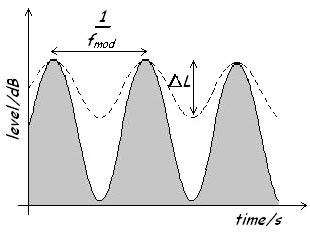
Fig 1: The effect of subjective duration on rapid amplitude modulated noise: (i) the modulation depth (unbroken line) and (ii) the perceived masking depth (dashed line).

Click on the links below to hear some noises which are rough compared with some that are not:

  Rough sound Not rough sound Broad band noise Amplitude modulated white noise White noise Tonal noise Amplitude modulated 1000 Hz tone  1000 Hz tone

In order to begin to construct a model for roughness we describe an amplitude modulated tone as a sound with a rapidly changing loudness level. To gain understanding of the effect on the ear of this rapidly changing level we must first understand the concept of subjective duration.

Subjective Duration

Usually the duration of a sound refers to the objective duration, and for sounds greater than 300 ms in length, this is adequate as the objective measurement and subjective perception are the same. However, as the duration of a sound gets shorter and goes below 300 ms a different subjective effect comes  into  play. Sounds of shorter durations are perceived to be longer than the objective measurement. For example, a sound of duration 10ms may be subjectively perceived to be 20 ms long and this has important consequences for the subjective perception of temporarily varying sounds, such as rough sounds.

How does this relate to roughness?

Returning to our amplitude modulated tone we can picture the changing level of the tone as the unbroken line in fig 1. But because the duration of a rapidly changing level appears subjectively to be longer, the level perceived by the ear does not drop as rapidly as the objectively measured level. So  the  perceived level only drops as low as delta L, indicated by the dashed line in fig 1.

To summarise, this means that the perceived masking depth is smaller than the objectively measured modulation depth. So the roughness of a sound can be evaluated from the following equation:

[R = cal cdot int_0^{24Bark}f_{_{mod}} cdot Delta Lcdot dz]

Where cal is a calibration factor,(f_{mod}) is the frequency of modulation and (Delta L) is the perceived masking depth [1].

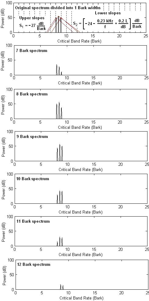
Fig 2: Diagram showing how Bark spectra 7 to 12 are obtained from the original spectrum

Because of the difficulty in accurately quantifying (Delta L), however, the roughness metric has not yet been standardised and there are several proposed methods of calculation. One method proposed by Aures [3] in 1985 requires the calculation of generalised modulation depths ((m^*_i)). First  the  signal is filtered into 24 individual 1 Bark wide bands. Next, the envelope of each filtered signal is multiplied by an appropriate weighting function in the frequency domain that gives maximal values at 70 Hz (in accordance with the behaviour of roughness). Then after conversion back to the time  domain  the r.m.s value of the each resulting time function is divided by the D.C. value of each original filtered signal to give 24 generalised modulation depths. These generalised modulation depths ((m^*_i)) are then each multiplied by a value (g(z_i)) where (z_i) is the Bark band  of  the signal. Each resulting value ((g(z_i) cdot m^*_i)) is equivalent to (f_{mod} cdot Delta L) for a particular Bark band so the equation above becomes:

[R = cal cdot sum_0^{24Bark} g(z_i) cdot m^*_i ]

Another difficult problem to overcome when developing a roughness algorithm is to get it to return low values of roughness for random sound such as white or pink noise. Aures achieved this by using the fact that the sound was divided up into Bark channels. The filtered spectrum within each Bark channel  can  be calculated using slopes devised by Terhardt [6] as shown in fig 2.

Calculation of the correlation coefficients between the envelopes of adjacent Bark bands gives small values for random sounds but large values if the amplitude modulation in adjacent channels is in phase. These values can be used to reduce the values of roughness for sounds such as white noise. Daniel  and  Weber [2] develop these ideas further in their algorithm for calculating roughness.

Widmann & Fastl [4] propose another method for calculation, using a measure of specific loudness made every 2 ms to calculate a time variable course of the masking pattern and from this a value for (Delta L) can be calculated. Jeong’s method [5] is another proposed method of calculation.

Fluctuation Strength

Fluctuation strength is similar in principle to roughness except it quantifies subjective perception of slower (up to 20Hz) amplitude modulation of a sound. The sensation of fluctuation strength persists up to 20Hz then at this point the sensation of roughness takes over. There is a fuzzy border at  the  change over of the two sensations when it is difficult to precisely quantify one or the other. Click on the links below to hear some noises which are fluctuating compared with some that are not:

  Fluctuating sound Not fluctuating sound Broad band noise Amplitude modulated white noise White noise Tonal noise Amplitude modulated 1000 Hz tone 1000 Hz tone

The unit of measure for fluctuation strength is the vacil. One vacil is defined as the fluctuation strength produced by a 1000Hz tone of 60dB which is 100% amplitude modulated at 4Hz. Maximal values are found to occur at a modulation frequency of 4 Hz. The following relation given by Fastl [1] shows  the  variation of fluctuation strength ((F)) with masking depth ((Delta L)), and modulation frequency ((f_{mod})):

[F = {0.008 cdot int_0^{24Bark} Delta L cdot dz over left({f_{_{mod}} over 4Hz}right) + left({4Hz over f_{_{mod}}}right) }]

It is important to note that (Delta L) represents the masking depth. This is not the same as the modulation depth, in this case, because of short term memory effects rather than post masking effects. Fluctuation strength has been used in applications such as to calculate an unbiased annoyance  metric.

References

[1] Zwicker E., Fastl H. ‘Psychoacoustics: Facts and Models’(1990).

[2] P. Daniel and R. Weber, “Psychoacoustic Roughness: Implementation of an Optimized Model,” Acustica 83, 113~123 (1997).

[3] W. Aures, “Ein Berechnungsverfahren der Rauhigkeit” (“A Procedure for Calculating Auditory Roughness”) Acustica 58, 268~281 (1985).

[4] U. Widmann and H. Fastl, “Calculating roughness using time-varying specific

loudness spectra,” Proc. Sound Quality Symposium ’98, 55~60 (1998).

[5] H. Jeong, “Sound quality analysis of nonstationary acoustic signals”, Ph. D. Thesis,

Department of Mechanical Engineering, Korea Advanced Institute of Science and

Technology (KAIST), 1999.

[6] E Terhardt “On the perceptions of periodic sound fluctuation (Roughness)” Acustica 30, 201, (1974).