Customised metrics
As discussed on previous pages, there are a considerable number of metrics in existance. A few of these are well defined, some even appear in standards, but many of the metrics in use are calculated using methods which are not disclosed. Many have experienced problems in relating the results of jury tests to the objective measures in the literature. The problem is that the objective measures that are freely available do not properly encompass the human response to sound. One solution to this is to use customized metrics which then only work for one specific product type. The problem is how to make such metrics. For this reason, a new method for developing such metrics is described here.
Consider the case study of the washing machine sounds. Furthermore, consider just the spin cycle. It was found that there was very weak correlation between the subjectively perceived quality and objective measurement of loudness, but the correlation was probably not statistically significant. (You can read more about this data by looking at the pages). Objective loudness, N, is an integeration of the specific loudnesses, N’, from 0 to 24 Bark:
[N = int_0^{24Bark} N’ dz ]
What if a weighting curve was used to alter this equation, to allow different frequency ranges to be emphasised or demphasised, would this lead to a better correlation? The equation would then become:
[N = int_{z=0}^{24} g(z)N’ dz ]
Where g(z) is the weighting function that is used. We shall refer to this as weighted loudness. There are various ways of finding the best weighting functions, and here we have used a iterative algorithm on a computer, and tasked the computer to find the best weighting function. This generic process is known as numerical optimisation and has been used widely in engineering.
An example of the final result obtained is shown in the following table. It shows the correlation coefficient between the subjective rating of quality and the standard objective loudness metric, and the new weighted loudness metric.
|
spin cycle
| ||||||||
| 1 | 2 | 3 | 4 | 5 | 6 | 7 |
Average | |
| Loudness, Eqn (1) | 0.33 | 0.74 | 0.64 | 0.69 | 0.84 | 0.78 | 0.80 | 0.65 |
| Weighted loudness, Eqn (2) | 0.99 | 0.89 | 0.94 | 0.94 | 0.99 | 0.93 | 0.95 | 0.95 |
The results show that with the weighting function, there is a significant correlation between the subjective response and the weighted loudness metric which wasn’t there before, with the average correlation coefficient going up from 0.65 to 0.95. In this case, the spin sound presented to the listener was chopped into 7 portions and we have objective measurements for these 7 portions, but only one overall subjective judgement for the spin cycle. We have looked for one weighting function g(z) which works best for all parts of the spin cycles, rather than a separate weighting function for each of the 7 parts.
How was the weighting function found?
The process is iterative:
- The computer randommly choses a starting weighting function, g(z).
- The weighted loudness, Nw, is found for each spin cycle using the weighting function, Eqn (2).
- Each of the weighted loudnesses, for each washing machine and each spin cycle, is correlated with the subjective responses for quality. This is done using a correlation coefficient.
- An average of the correlation coefficients multiplied by minus 1 is taken to form a figure of merit for the weighting function g(z). (The multiplication by -1 is done so the highest (best) correlation occurs when the figure of merit is a minimum).
- If the figure of merit is a minimum, then the best weighting function has been found and the process stops.
- Otherwise the weighting function g(z) is changed a little and we jump back to point 2.
So the computer keeps going around the loop, until the best weighting function is found. The figure below shows the best weighting function found in blue. Notice that some bandwidths are contributing positively to the weighted loudness, whereas others are being subtracted from the weighted loudness.
The blue curve contains 240 different weighting values, as the specific loudness is calculated at a resolution of 0.1 Bark. While it would be possible to allow the program to individually change all 240 values, it would not be very efficient or effective. There is a great risk that the data would be over-fitted and a very complex weighting function would result – a very exact fit for the data set used would be found, but it would work for no other washing machine. To mitigate against this a slow varying weighting function is best. Consequently, the parameters that the program changes are a smaller number of control points (marked by red squares). So the program has 5 different numbers it can change to form the weighting curve. The blue line is then formed from the red squares using a cubic spine interpolation. It might even be better if an even smaller number was used to ensure the best generalisation.
The computer program needs an inteligent way to move the red points to find the best positions. It is very inefficient ro try random guesses, and in complex problems a solution will never be found, instead an optimisation algorithm is used. This is an algorithm which can efficiently find minima in functions using the minimum number of attempts. There are many standard algorithms that can be used. Below is a chart of the figure of merit verses iteration number.
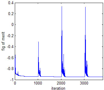
At the start (the left side of the graph), the figure of merit is quite large. After a 1000 times around the iteration loop, the figure of merit has reached a minimum and a best weighting function has been found. This process is repeated a number of times with a different starting guess for the initial weighting function, as is normal for numerical optimisation. The best result from the trials isused.
If you download this zip file, unzip it into a folder, you can see the coding used for this. If you want to run the programs, you’ll need to extract the two data files included as well. You need to run the file optimise.m.
By reviewing the specific loudness curves for the washing machines, and by examining the weighting function, it is possible to identify an important feature for preference:
The best washing machines (ACE) all have considerably lower energy at mid and higher Bark values (frequencies) than the poorer washing machines (BD). This is why the weighting curve shown previously has an emphasis on the weighting the mid-higher frequencies, because that is a determining feature. Indeed, as we are now weighting different frequency ranges in different ways, this metric probably has more in common with sharpness than it does with loudness. But the metric we have derived is more complex than sharpness, because some frequency ranges actually subtract from the weighted loudness.
What are the problems with this?
The results we present here are based on a very small number of machines (5). Would the weighting curve work for other machines not tested here? This is untested, but experience elsewhere would make us believe that more washing machines should be used in drawing up the weighting functions. Also, it is important not to use overly complex weighting functions, because then it is very likely that the results will be very specific to the data set used. Furthemore, the metric will only to work for washing machines, and it has lost it’s grounding in fundamental psychoacoustics. Such functions could never be standardised.
Having said this, very specialised and tailored metrics are the norm in automobile sound quality, and it is likely that until much more sophisticated auditory and perception models have been developed, that sound quality metrics are going to have to tailored for individual products for the foreseable future. The other solution is to forget about metrics and just use jury testing…